Usage as IPython Magics

This document was partially built from a notebook. Download it from GitHub (right-click to download).

Basic usage

First, you need to load the jupyter_tikz extension in your Jupyter Notebook. You can do this by running the following code cell:

%load_ext jupyter_tikz

Then, create a simple tikzpicture:

%%tikz
\begin{tikzpicture}
    \draw[help lines] grid (5, 5);
    \draw[fill=black] (1, 1) rectangle (2, 2);
    \draw[fill=black] (2, 1) rectangle (3, 2);
    \draw[fill=black] (3, 1) rectangle (4, 2);
    \draw[fill=black] (3, 2) rectangle (4, 3);
    \draw[fill=black] (2, 3) rectangle (3, 4);
\end{tikzpicture}

Finally, if you forget the usage, as for help by typing %tikz?, or visit additional options reference here.

%tikz?

%tikz [-as INPUT_TYPE] [-i] [-f] [-p LATEX_PREAMBLE] [-t TEX_PACKAGES]
            [-nt] [-l TIKZ_LIBRARIES] [-lp PGFPLOTS_LIBRARIES] [-nj] [-pj]
            [-pt] [-sc SCALE] [-r] [-d DPI] [-g] [-e] [-k] [-tp TEX_PROGRAM]
            [-ta TEX_ARGS] [-nc] [-s SAVE_TIKZ] [-st SAVE_TEX] [-sp SAVE_PDF]
            [-S SAVE_IMAGE] [-sv SAVE_VAR]
            [code]

Renders a TikZ diagram in a Jupyter notebook cell. This function can be used as both a line magic (%tikz) and a cell magic (%%tikz).

When used as cell magic, it executes the TeX/TikZ code within the cell:
    Example:
        In [3]: %%tikz
           ...:  \begin{tikzpicture}
           ...:     \draw (0,0) rectangle (1,1);
           ...: \end{tikzpicture}

When used as line magic, the TeX/TikZ code is passed as an IPython string variable:
    Example:
        In [4]: %tikz "$ipython_string_variable_with_code"

Additional options can be passed to the magic command to customize LaTeX code and rendering output:
    Example:
        In [5]: %%tikz -l=arrows,matrix
           ...: \matrix (m) [matrix of math nodes, row sep=3em, column sep=4em] {
           ...:     A & B \
           ...:     C & D \
           ...: };
           ...: \path[-stealth, line width=.4mm]
           ...:     (m-1-1) edge node [left ] {$ac$} (m-2-1)
           ...:     (m-1-1) edge node [above] {$ab$} (m-1-2)
           ...:     (m-1-2) edge node [right] {$bd$} (m-2-2)
           ...:     (m-2-1) edge node [below] {$cd$} (m-2-2);

positional arguments:
  code                  the variable in IPython with the Tex/TikZ code

options:
  -as INPUT_TYPE, --input-type INPUT_TYPE
                        Type of the input. Possible values are: `full-
                        document`, `standalone-document` and `tikzpicture`,
                        e.g., `-as=full-document`. Defaults to
                        `-as=standalone-document`.
  -i, --implicit-pic    Alias for `-as=tikzpicture`.
  -f, --full-document   Alias for `-as=full-document`.
  -p LATEX_PREAMBLE, --latex-preamble LATEX_PREAMBLE
                        LaTeX preamble to insert before the document, e.g.,
                        `-p "$preamble"`, with the preamble being an IPython
                        variable.
  -t TEX_PACKAGES, --tex-packages TEX_PACKAGES
                        Comma-separated list of TeX packages, e.g.,
                        `-t=amsfonts,amsmath`.
  -nt, --no-tikz        Force to not import the TikZ package.
  -l TIKZ_LIBRARIES, --tikz-libraries TIKZ_LIBRARIES
                        Comma-separated list of TikZ libraries, e.g.,
                        `-l=calc,arrows`.
  -lp PGFPLOTS_LIBRARIES, --pgfplots-libraries PGFPLOTS_LIBRARIES
                        Comma-separated list of pgfplots libraries, e.g.,
                        `-pl=groupplots,external`.
  -nj, --no-jinja       Disable Jinja2 rendering.
  -pj, --print-jinja    Print the rendered Jinja2 template.
  -pt, --print-tex      Print the full LaTeX document.
  -sc SCALE, --scale SCALE
                        The scale factor to apply to the TikZ diagram, e.g.,
                        `-sc=0.5`. Defaults to `-sc=1.0`.
  -r, --rasterize       Output a rasterized image (PNG) instead of SVG.
  -d DPI, --dpi DPI     DPI to use when rasterizing the image, e.g.,
                        `--dpi=300`. Defaults to `-d=96`.
  -g, --gray            Set grayscale to the rasterized image.
  -e, --full-err        Print the full error message when an error occurs.
  -k, --keep-temp       Keep temporary files.
  -tp TEX_PROGRAM, --tex-program TEX_PROGRAM
                        TeX program to use for compilation, e.g.,
                        `-tp=xelatex` or `-tp=lualatex`. Defaults to
                        `-tp=pdflatex`.
  -ta TEX_ARGS, --tex-args TEX_ARGS
                        Arguments to pass to the TeX program, e.g., `-ta
                        "$tex_args_ipython_variable"`.
  -nc, --no-compile     Do not compile the TeX code.
  -s SAVE_TIKZ, --save-tikz SAVE_TIKZ
                        Save the TikZ code to file, e.g., `-s filename.tikz`.
  -st SAVE_TEX, --save-tex SAVE_TEX
                        Save full LaTeX code to file, e.g., `-st
                        filename.tex`.
  -sp SAVE_PDF, --save-pdf SAVE_PDF
                        Save PDF file, e.g., `-sp filename.pdf`.
  -S SAVE_IMAGE, --save-image SAVE_IMAGE
                        Save the output image to file, e.g., `-S
                        filename.png`.
  -sv SAVE_VAR, --save-var SAVE_VAR
                        Save the TikZ or LaTeX code to an IPython variable,
                        e.g., `-sv my_var`.

Input type

You can generate TikZ pictures with different input formats by passing the -as=<input_type> (or --input-type=<input_type>) option. The available options are:

• full-document: Uses a full LaTeX document as input.
• standalone-document: Uses a standalone LaTeX document (with \documentclass{standalone}) and takes the content inside \begin{document} ... \end{document} as input.
• tikzpicture: Uses a standalone LaTeX document with the tikzpicture environment. It takes the content inside \begin{tikzpicture} ... \end{tikzpicture}.

If you don't specify the option, it uses the default: -as=standalone-document.

The code below shows an example using -as=full-document (the full-document input type):

%%tikz -as=full-document
\documentclass[tikz]{standalone}
\begin{document}
    \begin{tikzpicture}
        \draw[help lines] grid (5, 5);
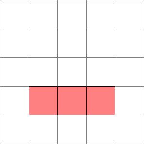
        \draw[fill=red] (1, 1) rectangle (2, 2);
        \draw[fill=red] (2, 1) rectangle (3, 2);
        \draw[fill=red] (3, 1) rectangle (4, 2);
        \draw[fill=red] (3, 2) rectangle (4, 3);
        \draw[fill=red] (2, 3) rectangle (3, 4);
    \end{tikzpicture}
\end{document}

Here is another example that uses -as=tikzpicture:

%%tikz -as=tikzpicture
\draw[help lines] grid (5, 5);
\draw[fill=magenta!10] (1, 1) rectangle (2, 2);
\draw[fill=magenta!10] (2, 1) rectangle (3, 2);
\draw[fill=magenta!10] (3, 1) rectangle (4, 2);
\draw[fill=magenta!10] (3, 2) rectangle (4, 3);
\draw[fill=magenta!10] (2, 3) rectangle (3, 4);

Tip

-as=<input_type> matches the initial substring of the input type. This means that both -as=full and -as=f are valid for setting the full-document input type.

The same rule applies to other types: for example, -as=s and -as=standalone for standalone-document, or -as=tikz and -as=t for tikzpicture.

Use this feature to reduce the amount of code you need to type. In the example below we are using -as=t to indicate tikzpicture:

%%tikz -as=t
\draw[help lines] grid (5, 5);
\draw[fill=magenta!10] (1, 1) rectangle (2, 2);
\draw[fill=magenta!10] (2, 1) rectangle (3, 2);
\draw[fill=magenta!10] (3, 1) rectangle (4, 2);
\draw[fill=magenta!10] (3, 2) rectangle (4, 3);
\draw[fill=magenta!10] (2, 3) rectangle (3, 4);

Aliases

Alternatively, you can use the aliases:

• -i (or --implicit-pic) for -as=tikzpicture
• -f (or --full-document) for -as=full-document

%%tikz -f
\documentclass[tikz]{standalone}
\begin{document}
    \begin{tikzpicture}
        \draw[help lines] grid (5, 5);
        \draw[fill=red] (1, 1) rectangle (2, 2);
        \draw[fill=red] (2, 1) rectangle (3, 2);
        \draw[fill=red] (3, 1) rectangle (4, 2);
        \draw[fill=red] (3, 2) rectangle (4, 3);
        \draw[fill=red] (2, 3) rectangle (3, 4);
    \end{tikzpicture}
\end{document}

Using preamble

You can set a preamble by using the flag -p="$<name_of_preamble>" (or --preamble="$<name_of_preamble>"). The preamble includes all LaTeX code before \begin{document}, except for the documentclass line.

Adding a preamble defining a custom color:

preamble = r"""
\usepackage{tikz}
\usepackage{xcolor}
\definecolor{my_color}{RGB}{0, 238, 255}
"""

Reuse the preamble in a standalone TeX document:

%%tikz -p "$preamble"
\begin{tikzpicture}
    \draw[help lines] grid (5, 5);
    \draw[fill=my_color] (1, 1) rectangle (2, 2);
    \draw[fill=my_color] (2, 1) rectangle (3, 2);
    \draw[fill=my_color] (3, 1) rectangle (4, 2);
    \draw[fill=my_color] (3, 2) rectangle (4, 3);
    \draw[fill=my_color] (2, 3) rectangle (3, 4);
\end{tikzpicture}

This also works with an implicit tikzpicture environment:

%%tikz -p "$preamble" -as=t
\draw[help lines] grid (5, 5);
\draw[fill=my_color] (1, 1) rectangle (2, 2);
\draw[fill=my_color] (3, 1) rectangle (4, 2);
\draw[fill=my_color] (2, 2) rectangle (3, 3);
\draw[fill=my_color] (3, 2) rectangle (4, 3);
\draw[fill=my_color] (2, 3) rectangle (3, 4);

Loading TeX packages and TikZ libraries

If you are not using the -f (or -as=full-document) flag, it's often useful to:

• Set the \usepackage{X,Y,Z} via --t=<X,Y,Z> (or --tex-packages=<X,Y,Z>)
• Set the \usetikzlibrary{X,Y,Z} via --l=<X,Y,Z> (or --tikz-libraries=<X,Y,Z>)
• Set the \usepgfplotslibrary{X,Y,Z} via -lp=<X,Y,Z> (or --pgfplots-libraries=<X,Y,Z>)

Tip

The tikz package is imported automatically, so it is not necessary to add in -t=tikz flag.

%%tikz -as=t -l=quotes,angles -t=amsfonts
% Example from Paul Gaborit
% http://www.texample.net/tikz/examples/angles-quotes/
\draw
    (3,-1) coordinate (a) node[right] {a}
    -- (0,0) coordinate (b) node[left] {b}
    -- (2,2) coordinate (c) node[above right] {c}
    pic["$\alpha$", draw=orange, <->, angle eccentricity=1.2, angle radius=1cm]
    {angle=a--b--c};

\node[rotate=10] (r) at (2.5, 0.65) {Something about in $\mathbb{R}^2$};

No TikZ

If you don't want to import the tikz package, you can use the flag -nt (or --no-tikz):

%%tikz -as=t -nt -t=pgfplots --pgfplots-libraries=statistics
\begin{axis}[
    title={Box Plot Example},
    boxplot/draw direction=y,
    ylabel={Values},
    xtick={1,2,3},
    xticklabels={Sample A, Sample B, Sample C},
]
% Sample A
\addplot+[
    boxplot prepared={
        median=3,
        upper quartile=4.5,
        lower quartile=2,
        upper whisker=6,
        lower whisker=1,
    },
] coordinates {};
\end{axis}

Scaling the output

You can scale the Tikz image using the -sc (or --scale) parameter(1):

1. It uses \boxscale from the graphicx package.

%%tikz -as=t -sc=2
\draw[help lines] grid (5, 5);
\draw[fill=black!10] (1, 1) rectangle (2, 2);
\draw[fill=black!10] (2, 1) rectangle (3, 2);
\draw[fill=black!10] (3, 1) rectangle (4, 2);
\draw[fill=black!10] (3, 2) rectangle (4, 3);
\draw[fill=black!10] (2, 3) rectangle (3, 4);

Which also works with standalone documents(1):

1. Not applicable with the -as=full-document input type.

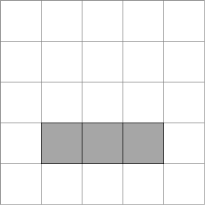
%%tikz -sc=0.75
\begin{tikzpicture}
    \draw[help lines] grid (5, 5);
    \draw[fill=black!50] (1, 1) rectangle (2, 2);
    \draw[fill=black!50] (2, 1) rectangle (3, 2);
    \draw[fill=black!50] (3, 1) rectangle (4, 2);
    \draw[fill=black!50] (3, 2) rectangle (4, 3);
    \draw[fill=black!50] (2, 3) rectangle (3, 4);
\end{tikzpicture}

Rasterizing the output

You can display the output as a rasterized (png) image by setting the -r (or --rasterize) parameter.

It is also possible to set the resolution (dots per inch) by using -d=<dpi_of_image> (or --dpi=<dpi_of_image>):

%%tikz -r --dpi=150
\begin{tikzpicture}
    \draw[help lines] grid (5, 5);
    \draw[fill=red!50] (1, 1) rectangle (2, 2);
    \draw[fill=red!50] (2, 1) rectangle (3, 2);
    \draw[fill=red!50] (3, 1) rectangle (4, 2);
\end{tikzpicture}

Setting to grayscale

When using a rasterized image, you can use the -g (or --gray) option to apply grayscale to the image. This is useful for previewing how printed versions will appear:

%%tikz -r --dpi=150 -g
\begin{tikzpicture}
    \draw[help lines] grid (5, 5);
    \draw[fill=red!50] (1, 1) rectangle (2, 2);
    \draw[fill=red!50] (2, 1) rectangle (3, 2);
    \draw[fill=red!50] (3, 1) rectangle (4, 2);
\end{tikzpicture}

Save to file

Save image to file

You can save the image output by setting -S=<name_of_image> (or --save-image=<name_of_image>)(1).

1. The magic automatically detects the output format. Including the file extension (.png or .svg) is optional.

For example, for saving an svg file in the path outputs/conway.svg(1):

1. You can specify folders by using the -S parameter (e.g., -S=outputs/file_name saves to ./outputs/conway.svg).

%%tikz --save-image=outputs/conway
\begin{tikzpicture}
    \draw[help lines] grid (5, 5);
    \draw[fill=black!50] (1, 1) rectangle (2, 2);
    \draw[fill=black!50] (2, 1) rectangle (3, 2);
\end{tikzpicture}

The output image will be saved in:

.
└─ outputs/
   └─ conway.svg

Save a rasterized image

For save a png file you should pass the option --rasterize:

%%tikz --save-image=outputs/conway.png --rasterize
\begin{tikzpicture}
    \draw[help lines] grid (5, 5);
    \draw[fill=black!50] (1, 1) rectangle (2, 2);
    \draw[fill=black!50] (2, 1) rectangle (3, 2);
\end{tikzpicture}

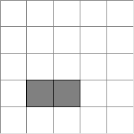
Which results in the following directory structure:

.
└─ outputs/
   └─ conway.svg
   └─ conway.png

Save TikZ code to file

You can save TikZ output by using -s=<tikz_file.tikz> (or --save-tikz=<tikz_file.tikz>)(1):

1. This command saves the cell content to a file.

%%tikz --save-image=outputs/a_dot -s=outputs/a_dot.tikz
\begin{tikzpicture}[scale=3]
    \draw (0,0) rectangle (1,1);
    \filldraw (0.5,0.5) circle (.1);
\end{tikzpicture}

Which results in the following directory structure:

.
└─ outputs/
   └─ a_dot.svg
   └─ a_dot.tikz

Save LaTeX code to file

If you want to save the full LaTeX code for use in an external IDE (e.g., TeXstudio), you can use -st=<tex_file> (or --save-tex=<tex_file.tex>):

%%tikz -st=outputs/a_dot.tex
\begin{tikzpicture}[scale=3]
    \draw (0,0) rectangle (1,1);
    \filldraw (0.5,0.5) circle (.1);
\end{tikzpicture}

.
└─ outputs/
   └─ a_dot.tex

Save PDF

You can even save PDF files using the flag -sp=<pdf_name.pdf> or --save-pdf=<pdf_name.pdf>:

%%tikz -sp=outputs/a_dot.pdf
\begin{tikzpicture}[scale=3]
    \draw (0,0) rectangle (1,1);
    \filldraw (0.5,0.5) circle (.1);
\end{tikzpicture}

.
└─ outputs/
   └─ a_dot.pdf

Input from other files

You can load figures from a file using the LaTeX command \input.

First, we are going to create a file named grid.tikz:

%%writefile grid.tikz
\draw [style=help lines, step=2]        (-1,-1) grid    (+7,+7);
\draw [line width=0.5mm, fill=blue!40!white]  (+2,+2) rectangle (+4,+4);

\draw [blue!60!white] (  2,  2) node[anchor=north east] {$(i  ,j  )$};
\draw [blue!60!white] (  4,  2) node[anchor=north west] {$(i+1,j  )$};
\draw [blue!60!white] (  4,  4) node[anchor=south west] {$(i+1,j+1)$};
\draw [blue!60!white] (  2,  4) node[anchor=south east] {$(i  ,j+1)$};

\filldraw [color=gray]  (0,0) circle (.1);
\filldraw [color=gray]  (0,2) circle (.1);
\filldraw [color=gray]  (0,4) circle (.1);
\filldraw [color=gray]  (0,6) circle (.1);
\filldraw [color=gray]  (2,0) circle (.1);
\filldraw [color=black] (2,2) circle (.1);
\filldraw [color=black] (2,4) circle (.1);
\filldraw [color=gray]  (2,6) circle (.1);
\filldraw [color=gray]  (4,0) circle (.1);
\filldraw [color=black] (4,2) circle (.1);
\filldraw [color=black] (4,4) circle (.1);
\filldraw [color=gray]  (4,6) circle (.1);
\filldraw [color=gray]  (6,0) circle (.1);
\filldraw [color=gray]  (6,2) circle (.1);
\filldraw [color=gray]  (6,4) circle (.1);
\filldraw [color=gray]  (6,6) circle (.1);

Overwriting grid.tikz

Then, load it using the \input command:

%%tikz -as=t
\input{grid.tikz}

PGFPlots with .tsv files

You can import external data using PGFPlots table {...}:

# import pandas as pd
# import numpy as np

# t = np.linspace(0,1)
# x = np.sin(2*np.pi*t)+0.1*np.random.rand(*t.shape)

# df = pd.DataFrame(dict(x=x), t).rename_axis(index='t')
# display(df.head(5))
# df.to_csv('data.tsv', sep=" ")

%%tikz -t=pgfplots -sc=2
\begin{tikzpicture}
    \begin{axis}[
        xlabel={$t$ (ms)},
        ylabel={Data},
        xmin=0, 
        xmax=1,
        ymin=-1.2, 
        ymax=1.2,
        xmajorgrids,
        ymajorgrids,
        title={PGFPlots graph with external data}
    ]
    \addplot [semithick, red] table {data.tsv};  % External data.tsv 
    \end{axis}
\end{tikzpicture}

Using IPython strings

Sometimes, you may want to generate a TikZ document from a string, rather than from cell content. You can do this using line magic.

conway_str = r"""\documentclass[tikz]{standalone}
\begin{document}
\begin{tikzpicture}
\draw[help lines] grid (5, 5);
\draw[fill=magenta] (1, 1) rectangle (2, 2);
\draw[fill=magenta] (2, 1) rectangle (3, 2);
\draw[fill=magenta] (3, 1) rectangle (4, 2);
\draw[fill=magenta] (3, 2) rectangle (4, 3);
\draw[fill=magenta] (2, 3) rectangle (3, 4);
\end{tikzpicture}
\end{document}"""

%tikz --input-type=f -S=cornway_image -s=conway_code.tex conway_str

Jinja templates

To help ensure that TikZ Pictures stay aligned with your data, you can use Jinja2 templates.

Tip

Since version 0.5, Jinja2 templates are enabled by default, so it's no longer necessary to use the -j flag. The jinja2 package is automatically installed during the installation of jupyter_tikz.

First, we need to populate some data:

node_names = "ABCDEF"
nodes = {s: int(365 / len(node_names) * i) for i, s in enumerate(node_names)}
n = len(nodes)
nodes

{"'A': 0, 'B': 60, 'C': 121, 'D': 182, 'E': 243, 'F': 304}

Since version 0.5, we have modified the standard Jinja2 syntax because {} braces clash with LaTeX. The table below shows the differences between the standard Jinja2 syntax and the Jupyter TikZ Jinja syntax:

Standard Jinja2 Syntax	Jupyter TikZ Syntax	Example
{{ expression }}	(* expression *)	\node at((* angle *):1);
{% logic/block %}	(** logic/block **)	(** for n1 in range(n) **)
{# comment #}	(~ comment ~)	(~ This won’t render ~)

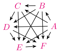
%%tikz -l=arrows,automata -sc=2
\begin{tikzpicture}[->,>=stealth',shorten >=1pt,auto,node distance=2.8cm, semithick]
  \tikzstyle{every state}=[fill=mymagenta,draw=none,text=white]

  % Nodes
  (** for name, angle in nodes.items() **)(~ For block ~)
    \node[color=magenta] (v(* loop.index0 *)) at ((* angle *):1) {$(* name *)$}; 
  (** endfor **)
  % Paths
  (** for n1 in range(n) **)
      (** for n2 in range(n) **)
          (** if n1 < n2 **)
            \path (v(* n1 *)) edge (v(* n2 *));
  (** endif **)
  (** endfor **)
  (** endfor **)
\end{tikzpicture}

It also works for full documents and implicit pictures:

%%tikz -as=f -r -d=200
\documentclass[tikz]{standalone}
\usetikzlibrary{arrows,automata}
\definecolor{mymagenta}{RGB}{226,0,116}
\begin{document}
\begin{tikzpicture}[->,>=stealth',shorten >=1pt,auto,node distance=2.8cm,
                    semithick]
  \tikzstyle{every state}=[fill=mymagenta,draw=none,text=white]

  (** for name, angle in nodes.items() **)
    \node[color=mymagenta] (v(* loop.index0 *)) at((* angle *):1) {$(* name *)$};
  (** endfor **)

  (** for n1 in range(n) **)
    (** for n2 in range(n) **)
        (** if n1 < n2 **)
            \path (v(* n1 *)) edge (v(* n2 *));
        (** endif **)
    (** endfor **)
  (** endfor **)
\end{tikzpicture}
\end{document}

Print Jinja

Sometimes, you'll make mistakes. Debugging transpiled code is challenging, especially without a mapping. To assist, you can print the Jinja rendered output using the -pj (or --print-jinja) flag (1):

1. The -pj printed code is also the source of the interpolated code.

Tip

Use a minus (-) before and/or after a block for whitespace control. For more information, refer to the Jinja2 documentation.

%%tikz -pj -l=arrows,automata -sc=2 --save-tex=outputs/jinja_rendered.tikz
\begin{tikzpicture}[->,>=stealth',shorten >=1pt,auto,node distance=2.8cm, semithick]
  \tikzstyle{every state}=[fill=mymagenta,draw=none,text=white]

  (~ Using minus `-` before/after each block to whitespace control. -~)
  (~- https://jinja.palletsprojects.com/en/3.0.x/templates/#whitespace-control -~)
  (** for name, angle in nodes.items() -**)
      \node[color=magenta] (v(* loop.index0 *)) at((* angle *):1) {$(* name *)$};
  (** endfor **)
  (** for n1 in range(n) -**)
  (** for n2 in range(n) -**)
  (**- if n1 < n2 -**)
    \path (v(* n1 *)) edge (v(* n2 *));
  (** endif -**)
  (** endfor -**)
(** endfor **)
\end{tikzpicture}

\begin{tikzpicture}[->,>=stealth',shorten >=1pt,auto,node distance=2.8cm, semithick]
  \tikzstyle{every state}=[fill=mymagenta,draw=none,text=white]

  \node[color=magenta] (v0) at(0:1) {$A$};
  \node[color=magenta] (v1) at(60:1) {$B$};
  \node[color=magenta] (v2) at(121:1) {$C$};
  \node[color=magenta] (v3) at(182:1) {$D$};
  \node[color=magenta] (v4) at(243:1) {$E$};
  \node[color=magenta] (v5) at(304:1) {$F$};

  \path (v0) edge (v1);
  \path (v0) edge (v2);
  \path (v0) edge (v3);
  \path (v0) edge (v4);
  \path (v0) edge (v5);
  \path (v1) edge (v2);
  \path (v1) edge (v3);
  \path (v1) edge (v4);
  \path (v1) edge (v5);
  \path (v2) edge (v3);
  \path (v2) edge (v4);
  \path (v2) edge (v5);
  \path (v3) edge (v4);
  \path (v3) edge (v5);
  \path (v4) edge (v5);

\end{tikzpicture}

Disabling Jinja rendering

If you don't want to use Jinja2 rendering you can tell it using the flag -nj (or --no-jinja):

%%tikz -nj -sc=2
\begin{tikzpicture}
    \node {(* Show `(*` because i'm not rendering Jinja*)};
\end{tikzpicture}

Exporting code to variables

With the flag -sv=<name_of_the_variable>, it is possible to save the code to an IPython string variable(1).

1. The code used to save to the variable is the same as that used by the -s flag.

In this example, we are going to save the code in the variable my_frame:

%%tikz -as=t -sv=my_frame
\draw (0,0) rectangle (1,1);

Now, we can reuse the variable in the code with Jinja:

%%tikz -as=t
\begin{tikzpicture}[scale=3]
    (* my_frame -*) % This is my_frame that I rendered before
    \filldraw (0.5,0.5) circle (.1);
\end{tikzpicture}

Combining with Jinja2

You can also combine -sv with Jinja blocks:

%%tikz -as=t -sv=node_names -sc=2
(** for name, angle in nodes.items() -**)
    \node[color=red] (v(* loop.index0 *)) at((* angle *):1) {$(* name *)$};
(** endfor -**)

Showing the content of variable node_names:

node_names

'\\node[color=red] (v0) at(0:1) {$A$};\n\\node[color=red] (v1) at(60:1) {$B$};\n\\node[color=red] (v2) at(121:1) {$C$};\n\\node[color=red] (v3) at(182:1) {$D$};\n\\node[color=red] (v4) at(243:1) {$E$};\n\\node[color=red] (v5) at(304:1) {$F$};\n'

Now, incorporate it into another tikzpicture:

%%tikz -l=arrows,automata -sc=2
\begin{tikzpicture}[->,>=stealth',shorten >=1pt,auto,node distance=2.8cm, semithick]
  \tikzstyle{every state}=[fill=mymagenta,draw=none,text=white]

  (* node_names *)

  (** for n1 in range(n) -**)
    (** for n2 in range(n) -**)
        (** if n1 < n2 -**)
            \path (v(* n1 *)) edge (v(* n2 *));
        (** endif **)
    (** endfor **)
  (** endfor **)
\end{tikzpicture}

Save preamble to variable

Finally, you can define a preamble using the -sv flag. Note that, because it is a preamble, you must avoid compiling it by using the option -nc (or --no-compile):

%%tikz -sv=my_preamble --no-compile
\usepackage{tikz}
\usepackage{xcolor}
\definecolor{mymagenta}{RGB}{226,0,116}

Reusing the preamble in the figure:

%%tikz -p "$my_preamble"
\begin{tikzpicture}
    \draw[help lines] grid (5, 5);
     \filldraw [color=mymagenta] (2.5,2.5) circle (1.5);
\end{tikzpicture}

TeX Program

You can change the TeX program using -tp=<tex_program> or --tex-program=<tex_program>:

%%tikz -as=tikz -t=pgfplots -nt -tp=lualatex
\begin{axis}[
  xlabel=$x$,
  ylabel={$f(x) = x^2 - x + 4$}
]
\addplot {x^2 - x + 4};
\end{axis}

Custom parameters

You can also pass custom parameters to the TeX program:

tex_params = "--enable-write18 --extra-mem-top=10000000"

%%tikz -as=tikz -t=pgfplots -nt -tp=pdflatex --tex-args "$tex_params"
\begin{axis}[
  xlabel=$x$,
  ylabel={$f(x) = x^2 - x +4$}
]
\addplot {x^2 - x +4};
\end{axis}

Logging and debugging

If you write invalid TikZ code, it will display the LaTeX command line error message(1):

1. Since LaTeX command line error messages tend to be verbose, by default, only the tail (last 20 lines) is shown.

%%tikz -as=t
% Error: Forgot Comma after the first coordinate
\draw[fill=black] (1, 1) rectangle (2, 2)

(%AppData%\Programs\MiKTeX\tex/latex/00miktex\epstopdf-sys.cfg))

! Package tikz Error: Giving up on this path. Did you forget a semicolon?.

See the tikz package documentation for explanation.
Type H for immediate help.
...

l.7 \end{tikzpicture}

?
! Emergency stop.
...

l.7 \end{tikzpicture}

! ==> Fatal error occurred, no output PDF file produced!
Transcript written on tikz.log.

Showing full error

If you want to see the entire error message, you can use the -e (or --full-error) option:

%%tikz -as=t -e
% Error: Comma after the first coordinate
\draw[fill=black] (1, 1) rectangle (2, 2)

This is pdfTeX, Version 3.141592653-2.6-1.40.26 (MiKTeX 24.4) (preloaded format=pdflatex.fmt) restricted \write18 enabled. entering extended mode (%AppData%/Local/Temp/tmp0l1mm2j8/tikz.tex LaTeX2e <2024-06-01> patch level 2 L3 programming layer <2024-05-27> (%AppData%\Local\Programs\MiKTeX\tex/latex/standalone\standalone.c ls Document Class: standalone 2022/10/10 v1.3b Class to compile TeX sub-files stan dalone (%AppData%\Local\Programs\MiKTeX\tex/latex/tools\shellesc.sty) (%AppData%\Local\Programs\MiKTeX\tex/generic/iftex\ifluatex.sty (%AppData%\Local\Programs\MiKTeX\tex/generic/iftex\iftex.sty)) (%AppData%\Local\Programs\MiKTeX\tex/latex/xkeyval\xkeyval.sty (%AppData%\Local\Programs\MiKTeX\tex/generic/xkeyval\xkeyval.tex (%AppData%\Local\Programs\MiKTeX\tex/generic/xkeyval\xkvutils.tex (%AppData%\Local\Programs\MiKTeX\tex/generic/xkeyval\keyval.tex))) ) (%AppData%\Local\Programs\MiKTeX\tex/latex/standalone\standalone.c fg) (%AppData%\Local\Programs\MiKTeX\tex/latex/base\article.cls Document Class: article 2023/05/17 v1.4n Standard LaTeX document class (%AppData%\Local\Programs\MiKTeX\tex/latex/base\size10.clo))) (%AppData%\Local\Programs\MiKTeX\tex/latex/pgf/frontendlayer\tikz. sty (%AppData%\Local\Programs\MiKTeX\tex/latex/pgf/basiclayer\pgf.sty (%AppData%\Local\Programs\MiKTeX\tex/latex/pgf/utilities\pgfrcs.st y (%AppData%\Local\Programs\MiKTeX\tex/generic/pgf/utilities\pgfutil -common.tex) (%AppData%\Local\Programs\MiKTeX\tex/generic/pgf/utilities\pgfutil -latex.def) (%AppData%\Local\Programs\MiKTeX\tex/generic/pgf/utilities\pgfrcs. code.tex (%AppData%\Local\Programs\MiKTeX\tex/generic/pgf\pgf.revision.tex) )) (%AppData%\Local\Programs\MiKTeX\tex/latex/pgf/basiclayer\pgfcore. sty (%AppData%\Local\Programs\MiKTeX\tex/latex/graphics\graphicx.sty (%AppData%\Local\Programs\MiKTeX\tex/latex/graphics\graphics.sty (%AppData%\Local\Programs\MiKTeX\tex/latex/graphics\trig.sty) (%AppData%\Local\Programs\MiKTeX\tex/latex/graphics-cfg\graphics.c fg) (%AppData%\Local\Programs\MiKTeX\tex/latex/graphics-def\pdftex.def ))) (%AppData%\Local\Programs\MiKTeX\tex/latex/pgf/systemlayer\pgfsys. sty (%AppData%\Local\Programs\MiKTeX\tex/generic/pgf/systemlayer\pgfsy s.code.tex (%AppData%\Local\Programs\MiKTeX\tex/generic/pgf/utilities\pgfkeys .code.tex (%AppData%\Local\Programs\MiKTeX\tex/generic/pgf/utilities\pgfkeys libraryfiltered.code.tex)) (%AppData%\Local\Programs\MiKTeX\tex/generic/pgf/systemlayer\pgf.c fg) (%AppData%\Local\Programs\MiKTeX\tex/generic/pgf/systemlayer\pgfsy s-pdftex.def (%AppData%\Local\Programs\MiKTeX\tex/generic/pgf/systemlayer\pgfsy s-common-pdf.def))) (%AppData%\Local\Programs\MiKTeX\tex/generic/pgf/systemlayer\pgfsy ssoftpath.code.tex) (%AppData%\Local\Programs\MiKTeX\tex/generic/pgf/systemlayer\pgfsy sprotocol.code.tex)) (%AppData%\Local\Programs\MiKTeX\tex/latex/xcolor\xcolor.sty (%AppData%\Local\Programs\MiKTeX\tex/latex/graphics-cfg\color.cfg) (%AppData%\Local\Programs\MiKTeX\tex/latex/graphics\mathcolor.ltx) ) (%AppData%\Local\Programs\MiKTeX\tex/generic/pgf/basiclayer\pgfcor e.code.tex (%AppData%\Local\Programs\MiKTeX\tex/generic/pgf/math\pgfmath.code .tex (%AppData%\Local\Programs\MiKTeX\tex/generic/pgf/math\pgfmathutil. code.tex) (%AppData%\Local\Programs\MiKTeX\tex/generic/pgf/math\pgfmathparse r.code.tex) (%AppData%\Local\Programs\MiKTeX\tex/generic/pgf/math\pgfmathfunct ions.code.tex) (%AppData%\Local\Programs\MiKTeX\tex/generic/pgf/math\pgfmathfunct ions.basic.code.tex) (%AppData%\Local\Programs\MiKTeX\tex/generic/pgf/math\pgfmathfunct ions.trigonometric.code.tex) (%AppData%\Local\Programs\MiKTeX\tex/generic/pgf/math\pgfmathfunct ions.random.code.tex) (%AppData%\Local\Programs\MiKTeX\tex/generic/pgf/math\pgfmathfunct ions.comparison.code.tex) (%AppData%\Local\Programs\MiKTeX\tex/generic/pgf/math\pgfmathfunct ions.base.code.tex) (%AppData%\Local\Programs\MiKTeX\tex/generic/pgf/math\pgfmathfunct ions.round.code.tex) (%AppData%\Local\Programs\MiKTeX\tex/generic/pgf/math\pgfmathfunct ions.misc.code.tex) (%AppData%\Local\Programs\MiKTeX\tex/generic/pgf/math\pgfmathfunct ions.integerarithmetics.code.tex) (%AppData%\Local\Programs\MiKTeX\tex/generic/pgf/math\pgfmathcalc. code.tex) (%AppData%\Local\Programs\MiKTeX\tex/generic/pgf/math\pgfmathfloat .code.tex)) (%AppData%\Local\Programs\MiKTeX\tex/generic/pgf/math\pgfint.code. tex) (%AppData%\Local\Programs\MiKTeX\tex/generic/pgf/basiclayer\pgfcor epoints.code.tex) (%AppData%\Local\Programs\MiKTeX\tex/generic/pgf/basiclayer\pgfcor epathconstruct.code.tex) (%AppData%\Local\Programs\MiKTeX\tex/generic/pgf/basiclayer\pgfcor epathusage.code.tex) (%AppData%\Local\Programs\MiKTeX\tex/generic/pgf/basiclayer\pgfcor escopes.code.tex) (%AppData%\Local\Programs\MiKTeX\tex/generic/pgf/basiclayer\pgfcor egraphicstate.code.tex) (%AppData%\Local\Programs\MiKTeX\tex/generic/pgf/basiclayer\pgfcor etransformations.code.tex) (%AppData%\Local\Programs\MiKTeX\tex/generic/pgf/basiclayer\pgfcor equick.code.tex) (%AppData%\Local\Programs\MiKTeX\tex/generic/pgf/basiclayer\pgfcor eobjects.code.tex) (%AppData%\Local\Programs\MiKTeX\tex/generic/pgf/basiclayer\pgfcor epathprocessing.code.tex) (%AppData%\Local\Programs\MiKTeX\tex/generic/pgf/basiclayer\pgfcor earrows.code.tex) (%AppData%\Local\Programs\MiKTeX\tex/generic/pgf/basiclayer\pgfcor eshade.code.tex) (%AppData%\Local\Programs\MiKTeX\tex/generic/pgf/basiclayer\pgfcor eimage.code.tex) (%AppData%\Local\Programs\MiKTeX\tex/generic/pgf/basiclayer\pgfcor eexternal.code.tex) (%AppData%\Local\Programs\MiKTeX\tex/generic/pgf/basiclayer\pgfcor elayers.code.tex) (%AppData%\Local\Programs\MiKTeX\tex/generic/pgf/basiclayer\pgfcor etransparency.code.tex) (%AppData%\Local\Programs\MiKTeX\tex/generic/pgf/basiclayer\pgfcor epatterns.code.tex) (%AppData%\Local\Programs\MiKTeX\tex/generic/pgf/basiclayer\pgfcor erdf.code.tex))) (%AppData%\Local\Programs\MiKTeX\tex/generic/pgf/modules\pgfmodule shapes.code.tex) (%AppData%\Local\Programs\MiKTeX\tex/generic/pgf/modules\pgfmodule plot.code.tex) (%AppData%\Local\Programs\MiKTeX\tex/latex/pgf/compatibility\pgfco mp-version-0-65.sty) (%AppData%\Local\Programs\MiKTeX\tex/latex/pgf/compatibility\pgfco mp-version-1-18.sty)) (%AppData%\Local\Programs\MiKTeX\tex/latex/pgf/utilities\pgffor.st y (%AppData%\Local\Programs\MiKTeX\tex/latex/pgf/utilities\pgfkeys.s ty (%AppData%\Local\Programs\MiKTeX\tex/generic/pgf/utilities\pgfkeys .code.tex)) (%AppData%\Local\Programs\MiKTeX\tex/latex/pgf/math\pgfmath.sty (%AppData%\Local\Programs\MiKTeX\tex/generic/pgf/math\pgfmath.code .tex)) (%AppData%\Local\Programs\MiKTeX\tex/generic/pgf/utilities\pgffor. code.tex)) (%AppData%\Local\Programs\MiKTeX\tex/generic/pgf/frontendlayer/tik z\tikz.code.tex (%AppData%\Local\Programs\MiKTeX\tex/generic/pgf/libraries\pgflibr aryplothandlers.code.tex) (%AppData%\Local\Programs\MiKTeX\tex/generic/pgf/modules\pgfmodule matrix.code.tex) (%AppData%\Local\Programs\MiKTeX\tex/generic/pgf/frontendlayer/tik z/libraries\tikzlibrarytopaths.code.tex))) (%AppData%\Local\Programs\MiKTeX\tex/latex/l3backend\l3backend-pdf tex.def) No file tikz.aux. (%AppData%\Local\Programs\MiKTeX\tex/context/base/mkii\supp-pdf.mk ii [Loading MPS to PDF converter (version 2006.09.02).] ) (%AppData%\Local\Programs\MiKTeX\tex/latex/epstopdf-pkg\epstopdf-b ase.sty (%AppData%\Local\Programs\MiKTeX\tex/latex/00miktex\epstopdf-sys.c fg)) ! Package tikz Error: Giving up on this path. Did you forget a semicolon?. See the tikz package documentation for explanation. Type H for immediate help. ... l.7 \end{tikzpicture} ? ! Emergency stop. ... l.7 \end{tikzpicture} ! ==> Fatal error occurred, no output PDF file produced! Transcript written on tikz.log.

Print entire LaTeX

If you want to print the entire LaTeX string for any reason, you can use the -pt (or --print-tex) option:

%%tikz -as=t -sc=2 --print-tex
\draw[help lines] grid (5, 5);
\draw[fill=black!10] (1, 1) rectangle (2, 2);
\draw[fill=black!10] (2, 1) rectangle (3, 2);
\draw[fill=black!10] (3, 1) rectangle (4, 2);
\draw[fill=black!10] (3, 2) rectangle (4, 3);
\draw[fill=black!10] (2, 3) rectangle (3, 4);

\documentclass{standalone}
\usepackage{graphicx}
\usepackage{tikz}
\begin{document}
    \scalebox{2.0}{
    \begin{tikzpicture}
        \draw[help lines] grid (5, 5);
        \draw[fill=black!10] (1, 1) rectangle (2, 2);
        \draw[fill=black!10] (2, 1) rectangle (3, 2);
        \draw[fill=black!10] (3, 1) rectangle (4, 2);
        \draw[fill=black!10] (3, 2) rectangle (4, 3);
        \draw[fill=black!10] (2, 3) rectangle (3, 4);
    \end{tikzpicture}
    }
\end{document}

Finally, you can keep the temporary files (LaTeX, PDF and image) for further investigation by using -k (or --keep). The file names are hex representation of hash of the full LaTeX code.

%%tikz -as=t -sc=2 -k
\draw[help lines] grid (5, 5);
\draw[fill=black!10] (1, 1) rectangle (2, 2);
\draw[fill=black!10] (2, 1) rectangle (3, 2);
\draw[fill=black!10] (3, 1) rectangle (4, 2);
\draw[fill=black!10] (3, 2) rectangle (4, 3);
\draw[fill=black!10] (2, 3) rectangle (3, 4);

Which results in the following directory structure:

.
└─ outputs/
   └─ 7f91d338e3919e6dafebb8c59a160504.aux
   └─ 7f91d338e3919e6dafebb8c59a160504.log
   └─ 7f91d338e3919e6dafebb8c59a160504.pdf
   └─ 7f91d338e3919e6dafebb8c59a160504.svg